Task tracking is essential for managing projects effectively, and Google Sheets provides a simple yet powerful way to keep track of your tasks. One of the most useful features in Google Sheets for task tracking is the ability to create filters. Filters allow you to sort and view specific data, making it easier to manage tasks, prioritize work, and keep everything organized. In this blog post, we will guide you through the process of creating a filter in Google Sheets, with easy-to-follow steps and examples.
Step 1: Set Up Your Task Tracking Spreadsheet
Before creating a filter, you need to set up a task tracking spreadsheet. Here’s how:
- Open Google Sheets: Start by opening Google Sheets and creating a new spreadsheet.
- Create Task Columns: In your spreadsheet, create columns for the information you want to track. Common columns for task tracking include:
- Task Name
- Due Date
- Priority
- Status
- Assigned To
- Enter Your Tasks: Fill in the rows with your tasks and their respective details. Your spreadsheet might look something like this:
| Task Name | Due Date | Priority | Status | Assigned To |
|---|---|---|---|---|
| Write Blog Post | 2024-09-01 | High | In Progress | John Doe |
| Update Website | 2024-09-05 | Medium | Not Started | Jane Smith |
| Design Logo | 2024-09-07 | High | Completed | Mark Brown |
Step 2: Apply a Filter
Now that your task list is ready, it’s time to apply a filter so you can view and manage your tasks more efficiently.
- Select the Header Row: Click on the header row of your spreadsheet (the row with the column names).
- Apply the Filter:
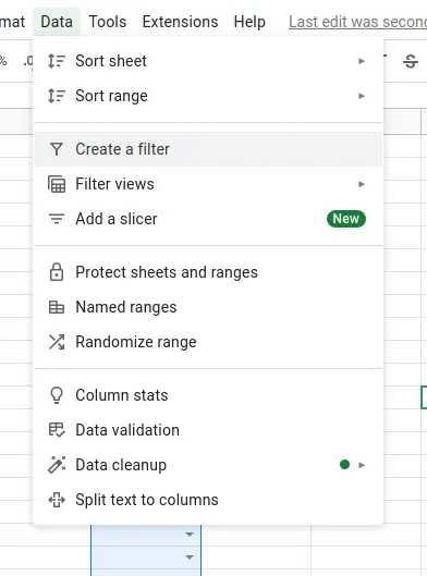
- Go to the top menu and click on “Data”.
- From the dropdown menu, select “Create a filter”. This will add a filter icon (a small funnel) to each header.
- Filter Your Tasks:
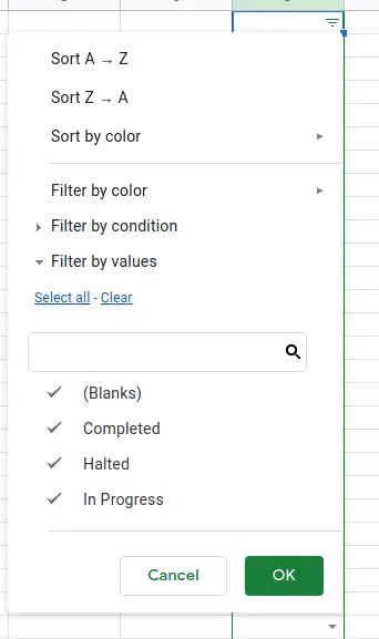
- Click on the filter icon in the column you want to filter by. For example, if you want to see only the tasks that are “High” priority, click on the filter icon in the “Priority” column.
- Uncheck all other options, leaving only “High” checked, then click “OK”.
- Your spreadsheet will now display only the tasks with a “High” priority.
Step 3: Use Multiple Filters for Advanced Task Management
You can apply multiple filters to narrow down your task list even further. For example, you can filter by both “High” priority and tasks that are “In Progress” to see only the most urgent tasks that need attention.
- Apply Additional Filters:
- After filtering by priority, click on the filter icon in the “Status” column.
- Select “In Progress” and click “OK”.
- Now, you will see only the tasks that are both high priority and currently in progress.
This functionality allows you to focus on specific tasks based on various criteria, making task management more efficient and tailored to your needs.
Step 4: Save and Share Your Filtered View
Once you’ve set up your filters, you can save the view or share it with your team.
- Save the Filter:
- You can save the filtered view by clicking on “Data” > “Filter views” > “Save as filter view”.
- Name your filter view, and it will be saved for future use.
- Share the Filtered Spreadsheet:
- To share the filtered spreadsheet with others, click on the “Share” button in the top-right corner.
- Enter the email addresses of the people you want to share with, and set the appropriate permissions (Viewer, Commenter, or Editor).
- Click “Send” to share the filtered view.
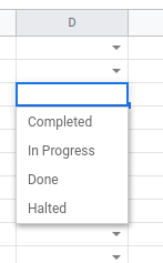
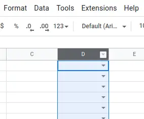
Another Example as we can see in Images, as below
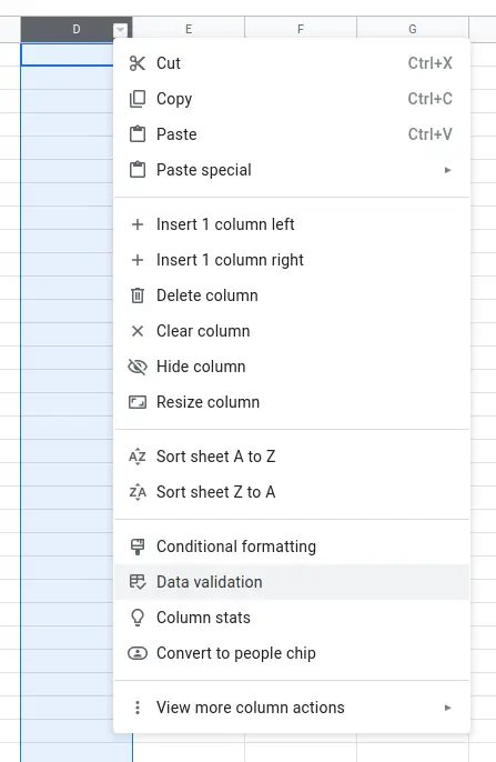
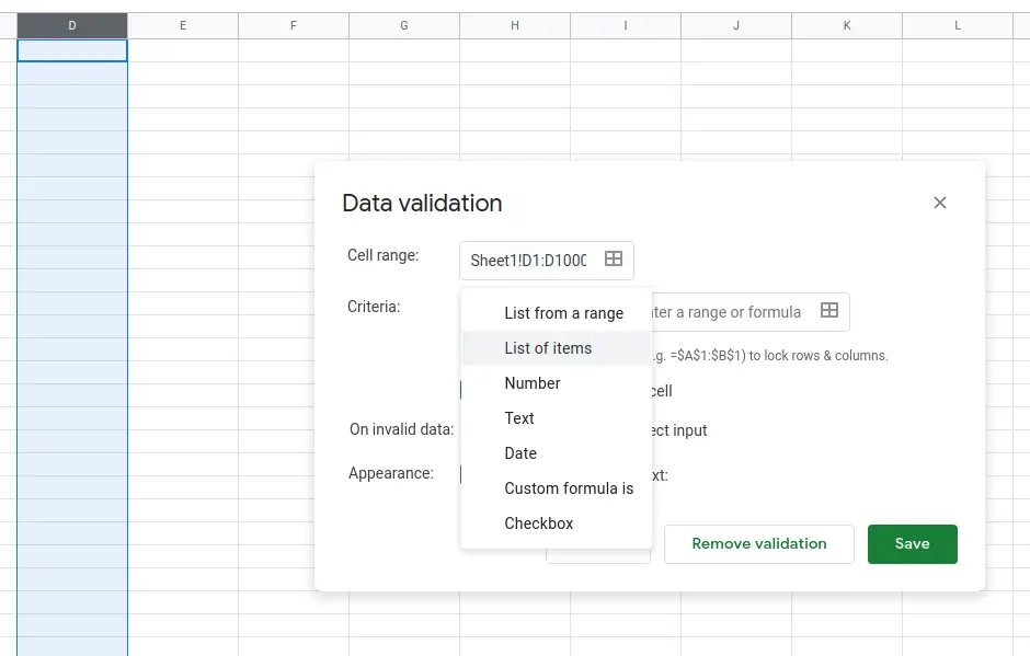
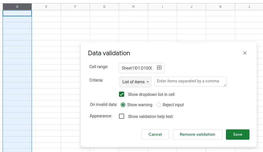
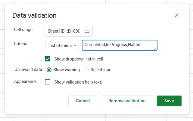
Creating filters in Google Sheets is a powerful way to manage your tasks effectively. Whether you’re working on a personal project or collaborating with a team, filters help you focus on the most important tasks and keep everything organized. By following the steps outlined in this guide, you’ll be able to set up a task tracking system in Google Sheets that works for you.